Melissa Kenney1, Michael Gerst2, Toni Viskari3, Austin Delaney4, Freya Olsson4, Carl Boettiger5, Quinn Thomas4
1University of Minnesota, 2University of Maryland, 3Finnish Meteorological Institute,4Virginia Tech, 5University of California, Berkeley
With the growth of the EFI NEON Ecological Forecasting Challenge, we have outgrown the current Challenge Dashboard, which was designed to accommodate a smaller set of forecasts and synthesis questions. Thus, we have reenvisioned the next stage of the EFI-RCN NEON Forecast Challenge Dashboard in order to facilitate the ability to answer a wider range of questions that forecast challenge users would be interested in exploring.
The main audience for this dashboard are NEON forecasters, EFI, Forecast Synthesizers, and students in classes or teams participating in the Forecast Challenge. Given this audience, we have identified 3 different dashboard elements that will be important to include:
forecast synthesis overview,
summary metrics about the Forecast challenge, and
self diagnostic platform.
During the June 2023 Unconference in Boulder, our team focused on scoping all three dashboard elements and prototyping the forecast synthesis overview. The objective of the synthesis overview visual platform is to support community learning and emergent theory development. Thus, the synthesis visualizations are aimed at creating a low bar entry for multi-model exploration to understand model performance, identify characteristics that lead to stronger performance than others, the spatial or ecosystems that are more predictable, and temporal forecast validity.
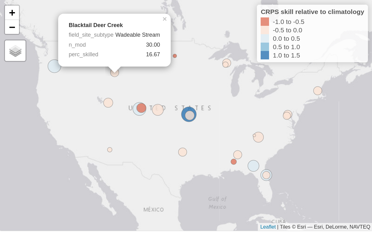
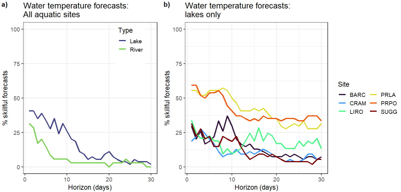
You can view the prototype developed during the meeting HERE and in Figures 1 and 2.
Figure 1. Static image of an interactive map of aggregate forecast skill relative to climatology at each forecasted sites, here showing the water temperature forecasts for the aquatics theme. Bubble colour represents the continuous rank probability score (CRPS) skill relative to climatology with positive values (blues) showing submitted models on average perform better than climatology and negative values showing submitted models perform worse (reds). The size of the bubble represents the percentage of submitted models that outperformed the climatology null (i.e., larger sized bubbles have a higher percentage of skilled models). When hovered over, the bubbles show this percentage (perc_skilled), the site type (field_site_subtype), as well as the total number of models forecasting at that site (n_mod).
Figure 2. a) Percentage of submitted models that are classed as ‘skillful’ (outperform the null climatology forecast based on the continuous rank probability score metric) at the river (n=27) and lake sites (n=6) for water temperature forecasts at each horizon from 1 to 30 days ahead. b) Percentage of submitted models that are classed as ‘skillful’ for water temperature forecasts at six of the lake sites (https://www.neonscience.org/field-sites/explore-field-sites).
Developing these graphics requires aggregation of skill scores.There are a multitude of metrics that can be used to calculate the skill score, which each have their own benefits and flaws. Thus, there should be multiple skill scores for different metrics with clear presentation of what metric is used at a given visualization. Additionally, in order to isolate what sites are more interesting from a model development perspective, there needs to be a comparison of how many of the models meet a baseline skill score at a given site at a chosen time frame. That allows isolating challenge areas and also easily informs which models really succeed at situations where others struggle. For better future analysis of how models perform at certain sites, we also envisage the visualization to include the skill scores for the relevant drivers (NOAA weather) for comparison. For example, if we see a drop in skill across models in water temperature projections after some time, there should be a direct method to assess if this reflects overall flawed model dynamics or if the weather forecast driving the water temperature loses its reliability. This also allows the user to approximate a maximum length in which the model performance analysis is at all useful.
In addition to the main synthesis overview, the goal of this platform is to support exploration of synthesis data. For all themes, there was general agreement that it would be useful to pull up at a glance, site characteristics, a photo, and basic summary statistics about the number of models and model performance.
During the meeting, we worked with the Aquatics and Beetles Challenge teams to identify some of the key data aggregation groupings that will be important to facilitate exploration. One important distinction arose during the conversations – the baseline model, time scale, and data latency. For Aquatics there is a long time series of data that create a climatology and data are provided relatively quickly via data loggers. For Beetles, there is a different null baseline model given the length of historic data that is different at each site and it takes a year to provide beetle abundance and richness assessment. There was also a desire to have specific types of synthesis visualizations including the species accumulation curve over years, 3-year running average, and indicating the lower and upper bounds of a particular variable (use in scale). Thus, for both Beetles and Aquatics there are similarities and differences in the types of groupings that would be most useful to support synthesis exploration.
Table 1. Different data groupings that would be useful to facilitate easy-to-develop synthesis visualizations of the EFI-NEON Forecast Challenge models to facilitate learning and community theory development.
Groupings
All Themes
Aquatics
Beetles
Team / Challenge
theme, site, model ID, customized classroom or team groupings
particular variables (e.g., DO) within a theme
Spatial / Ecosystems
sites, NEON domains, site type (river, stream, lake…), altitude (high vs lowlands)
sites by distance, dominant NLCD classification
Temporal Scale
average for past year, seasonal groupings,
1 day, 5 days, 7 days, 15 days, 30 days
14 days, growing season, multi-year (up to 5 year) forecasts
Models
best model at each site, model inputs, model structure, functional type, output uncertainty representation
model run time, model computational requirements
Skill Scoring
current skill forecast approaches, better than climatology/null baseline,
comparison of your model to the best forecast
Other Features
environmental variables and weather forecast observations
comparison with weather/climate forecast skill
disturbance events (e.g., widlfire), growing season dates at each sites, site disturbance characteristics (e.g., mowing, fencing)
In addition to the synthesis overview, there were two complementary and linked platforms that will create the dashboard. First, the objective of the forecast challenge overview is to provide a basic summary of metrics related to the overall EFI NEON Ecological Forecasting Challenge. Specifically, the metrics that would be included are: number of forecasts submitted, number of unique teams, percentage (or median of all) of models that are better than climatology or a null model per theme, and total forecast and observation pairs.
Second, the objective of the self-diagnositic platform is to provide an overview for individuals or team forecast contributions and performance. The types of summaries that will be provided for the forecasters are: confirmation of forecast submission, date of the most recent forecast submitted for a model, model performance relative to climatology or null model, model prediction versus observation, model performance vs other selected models, and model skill over a specific time horizon (to assess whether it performs better over time).
Overall, the goal of the re-envisioned visual dashboard is to create platforms that will allow us to track challenge engagement, individually or as a team diagnose any model submission problems and performance improvement opportunities, and support community theory development through a synthesis given the range of models submitted through the EFI NEON Ecological Forecasting Challenge. Long-term, if this platform structure is useful and robust, it could be applied to other systems where there are multi-model predictions and there is a desire to collaboratively learn together to improve our theoretical understanding and forecasts to support decision-making.
We are looking for input from the EFI community on the synthesis dashboard for other themes, to discuss with individuals what synthesis would be most relevant to phenology, terrestrial, and ticks forecasters. Reach out to info@ecoforecast.org to share your thoughts or let us know you would like to join future conversations about updating the dashboard.
Post by: Kelsey Yule; Project Manager, NEON Biorepository and Nico Franz; Principal Investigator, NEON Biorepository
Background. The National Ecological Observatory Network (NEON; https://www.neonscience.org/) is known for producing and publishing 180 (and counting) data products that are openly available to both researchers and the greater public. These data products span scales: individual organisms to whole ecosystems, seconds to decades, and meters to across the continent. They are proving to be a central resource for addressing ecological forecasting challenges. Less well known, however, is that these data products are all either directly the result of or spatially and temporally linked to NEON sampling of physical biological (e.g. microbial, plant, animal) and environmental (e.g. soil, atmospheric deposition) samples at all 81 NEON sites.
The NEON Biorepository at Arizona State University (Tempe, AZ) curates and makes available for research the vast majority of these samples, which consist of over 60 types and number over 100,000 per year. Part of the ASU Biodiversity Knowledge Integration Center and located at the ASU Biocollections, the NEON Biorepository was initiated in late 2018 and has received nearly 200,000 samples to date (corresponding to some 850 identified taxa in our reference classification). Sampling strategies and preservation methods that have resulted in the catalog of NEON Biorepository samples have been designed to facilitate their use in large scale studies of the ecological and evolutionary responses of organisms to change. While many of these samples, such as pinned insects and herbarium vouchers, are characteristic of biocollections, others are atypical and meant to serve researchers who may not have previously considered using natural history collections. These unconventional samples include: environmental samples (e.g. ground belowground biomass and litterfall, particulate mass filters; tissue, blood, hair and fecal samples; DNA extractions; and bulk, unidentified community-level samples (e.g. bycatch from sampling for focal taxa, aquatic and terrestrial microbes). Within the overarching NEON program, examination of these freely available NEON Biorepository samples is the path to forecasting some phenomena, such as the spread of disease and invasive species in non-focal taxonomic groups.
NEON Biorepository samples include: pinned, identified insects; dry soils; bulk, unidentified, ground-dwelling invertebrate community samples; frozen small mammal tissue samples
Sample Use. Critically, the NEON Biorepository can be contrasted with many other biocollections in the allowable and encouraged range of sample uses. For example, some sample types are collected for the express purpose of generating important datasets through analyses that necessitate consumption and even occasionally full destruction. Those of us at the NEON Biorepository are working to expedite sample uptake as early and often as possible. While we hope to maintain a decadal sample time series, we also recognize that the data potential inherent within these samples needs to be unlocked quickly to be maximally useful for ecological forecasting and, therefore, to decision making.
Data portal. In addition to providing access to NEON samples, the NEON Biorepository publishes biodiversity data in several forms on the NEON Biorepository data portal (https://biorepo.neonscience.org/portal/index.php). Users can interact with this portal in several ways: learn more about NEON sample types and collection and preservation methods; search and map available samples; download sample data in the form of Darwin Core records; find sample-associated data collected by other researchers; explore other natural history collections’ data collected from NEON sites; initiate sample loan requests; read sample and data use policies; and contribute and publish their own value-added sample-associated data. While more rapidly publishable NEON field data will likely be a first stop for forecasting needs, the NEON Biorepository data portal will be the only source for data products arising from additional analyses of samples collated across different research groups.
Map results for the spatial and taxonomic distribution of NEON mosquito (Culicidae) specimens currently available for use
Exploration of feasible forecasting collaborations. The NEON Biorepository faces both opportunities and challenges as it navigates its role in the ecological forecasting community. As unforeseen data needs arise, the NEON Biorepository will provide the only remaining physical records allowing us to measure relevant prior conditions. Yet, we are especially keen to collaboratively explore what kinds of forecasting challenges are possible to address now,particularly with regards to biodiversity and community level forecasts. And for those that are not possible now, what is missing and how can we collaborate to fill gaps in raw data and analytical methods? Responses to future forecasting challenges will be strengthened by understanding these parameters as soon as possible. We at the NEON Biorepository actively solicit inquiries by researchers motivated to tackle these opportunities, and our special relationship to NEON Biorepository data can facilitate these efforts. Please contact us with questions, suggestions, and ideas at biorepo@asu.edu.
Date: April 20, 2020, updated June 29, 2020and December 16, 2022
For individuals new to the field of ecological forecasting it can feel like there are an overwhelming number of methods and tools to learn and implement. On the other hand, individuals who have been forecasting for some time may want to know if there are any additional tools that others have found useful. In a series of 4 blog posts, the Methods and Cyberinfrastructure EFI Working Groups will highlight common tasks in ecological forecasting and methods and tools to help with those tasks.
Modeling & Statistical resources, including Uncertainty Quantification & Propagation
Data Ingest, Cleaning, and Management
Visualization, Decision Support, and User Interfaces.
The tasks and associated tools will be included in each of the four blog posts as well as kept on easily accessible and periodically updated web pages linked off the EFI Resources, Methods & Tools, and Cyberinfrastructure pages.
Resources and tools listed in the four categories of tasks are meant to be living documents. This list is not meant to be a comprehensive overview of all possible resources, as there are some tasks where there are hundreds of different tools available. Instead we focus on commonly used tools. However, if there are often used tools and resources we are missing, we welcome input from anyone — suggestions can be shared using this Google Form.
On the short-term scale, our goal is to provide the Task Views as resources to the ecological forecasting community. In the long-term, we want to supplement these resources with gap analyses to determine where there are unmet needs for generalizable tools (i.e. methods are known but tools don’t exist) versus where methods don’t exist and there’s a need for new research on statistical methods or cyberinfrastructure.
Curators: Jacob Zwart1, Alexey Shiklomanov2, Kenton McHenry3, Daniel S. Katz3, Rob Kooper3, Carl Boettiger4, Bryce Mecum5, Michael Dietze6, Quinn Thomas7
1USGS, 2NASA, 3National Center for Supercomputing Applications at the University of Illinois Urbana-Champaign, 4University of California, Berkeley, 5National Center for Ecological Analysis and Synthesis, 6Boston University, 7Virginia Tech
Reproducibility8 of scientific output is of utmost importance because it builds trust between stakeholders and scientists, increases scientific transparency, and often makes it easier to build upon methods and/or add new data to an analysis. Reproducibility is particularly critical when forecasting, because the same analyses need to be repeated again and again as new data become available, often in an automated workflow. Furthermore, reproducible workflows are essential to benchmark forecasting skill, improve ecological models, and analyze trends in ecological systems over time. All forecasting projects, from single location forecasts disseminated to only a few stakeholders to daily-updating continental-scale forecasts for public consumption, benefit from using tools and techniques that enable reproducible workflows. However, the project size often dictates which tools are most appropriate, and here we give a brief introductory overview of some of the tools available to help make your ecological forecast reproducible. There are many more tools available than what we describe here, and we primarily focus on open-source software to facilitate reproducibility independent of software access.
8Reproducibility is the degree of agreement among results generated by at least two independent groups using the same suite of methods. Many of the tools highlighted here facilitate repeatability, which is a measure of agreement among results from a single task that is performed by the same person or tool. Repeatability is necessary for reproducible forecasting workflows.
Scripted Analyses
Forecasts produced without using scripted analyses are often inefficient and prone to non-reproducible output. Therefore, it is best to perform data ingest and cleaning, modeling, data assimilation, and forecast visualization using a scripted computing language that perform tasks automatically once properly configured.
Interpreted languages allow the user to execute commands line-by-line, interactively, in real time. This makes debugging and exploratory analysis much easier, and significantly reduces programmer time for performing analyses. Analyses using interpreted languages are also usually easier to reproduce because of fewer installation/configuration steps (and more standardized, centralized installation mechanisms). This convenience generally comes at the expense of computational speed, but many times the tradeoff is worth it.
R – Originally developed for statistical computing, and still primarily used for data science and other scientific computing tasks. Many important data science tools, including statistical distributions, plotting, and tabular data analysis, are included in the core language. Tens of thousands of add-on packages for just about any task imaginable exist.
Python – General purpose programming language with a much more limited set of core features than R. Many data-science features are accessible through add-on packages and are curated through repositories such as PyPi, Anaconda, and Enthought.
Julia – Very recent language. Claims to combine the ease-of-use of interpreted languages like R and Python with the performance of compiled languages like C and Fortran. Specifically relevant to forecasting and uncertainty propagation, Julia has extremely powerful probabilistic programming tools (e.g. Turing for Bayesian inference, Flux for machine learning).
Compiled languages generally perform computationally intensive tasks much faster (up to 80x or more) than interpreted languages. However, their syntax is generally stricter / less forgiving, and analyses have to be written as complete programs that are compiled in operating system-specific (and even machine-specific) ways. In general, these languages should be avoided in favor of easier-to-use interpreted languages unless you are addressing specific computational bottlenecks. Note that all of the interpreted languages above provide ways to call specific functions/subroutines written in these compiled languages, so you have the option to only use these routines for specific, computationally-limiting steps in your analysis. Commonly used compiled languages include:
A good standard is to develop an analysis using an interpreted language first and assess if it is fast enough for your needs. If it is fast enough, then you are done! If not, do some basic profiling to identify performance bottlenecks. See if there are existing tools or techniques in the language you are using that can help address the bottlenecks. Only fall back on compiled languages if you’ve reasonably exhausted possibilities using your current language.
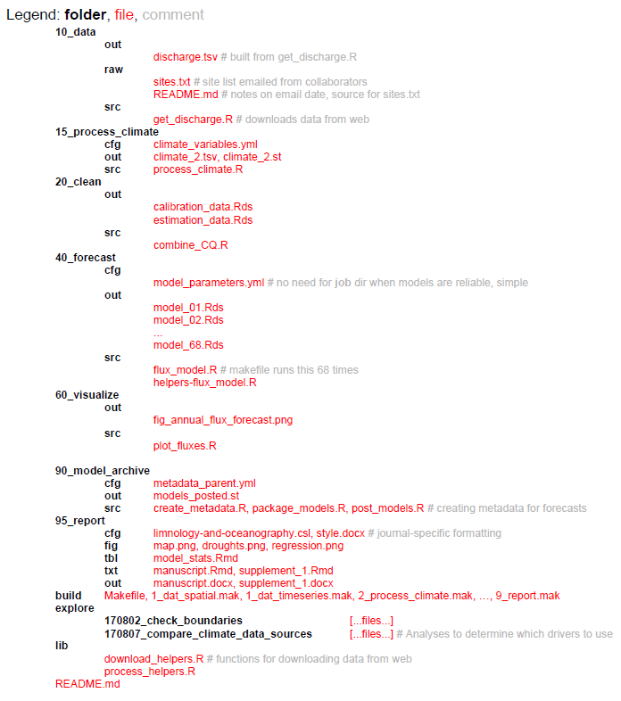
Organized project structures help the scientist and collaborators navigate the workflow of the ecological forecasting project from data input to dissemination of results. Subfolders should be used to break up the project into conceptually distinct steps of the forecasts and sequentially numbering of scripts and subfolders helps with readability, for example, “10_data”, “20_clean”, “40_forecast”, “60_visualize”, “95_report” (see more detailed example below). The number prefixes should represent a conceptual workflow for each forecasting project, and subdirectories within each phase of the project should describe the inputs, outputs, and functions for each step. Generally, unnumbered directories should contain supporting files that apply to the overall project, for example a configuration file that is used in multiple phases of the forecasting project.
Example of organized folder and file structure for a forecasting project.
Tools for organized project structures
Project-oriented workflows are self-contained workflows enabling reproducibility and navigability when used in conjunction with organized project structures for ecological forecasting projects. Ideally, a collaborator should be able to run the entire project without changing any code or files (e.g. file paths should be workstation-independent). R and Python both have options for enabling self-contained workflows in their coding environments.
R – RStudio projects – R projects allow for analyses to be contained in a single working directory that can be given to a collaborator and run without changing file directory paths.
Python – Spyder projects – Python projects also allow for self-contained analyses and integration with Git version control (see Version Control below).
Version control is the process of managing changes in code and workflows and improves transparency in the code development process and facilitates open science and reproducibility. Code versioning also enables experimentation and development of code on different “branches” while retaining canonical files that can be used in operations, for example. Modern version control systems make it easy to create and switch between branches within a code base, encouraging developers to experiment without potentially breaking changes without worrying about losing stable code. This is especially useful for forecasting projects that need to make forecasts at regular schedules (e.g. daily), while researchers can also make alterations to the code base on experimental branches. Finally, version control facilitates collaboration by formalizing the process for introducing changes and keeping a record of who introduced which changes, when, and why. Additionally, version control allows contributions in an open way from even unknown contributors with the opportunity for the main authors control which contributions are accepted. Software development is a trillion dollar industry and it is well worth the time learning the basics of industry standard tools like version control, rather than relying on ad hoc and error prone approaches such as file naming (e.g. script.v2.R, python_script_final_FINAL.py), Dropbox/Google Drive, or emailing files to collaborators.
Tools for version control
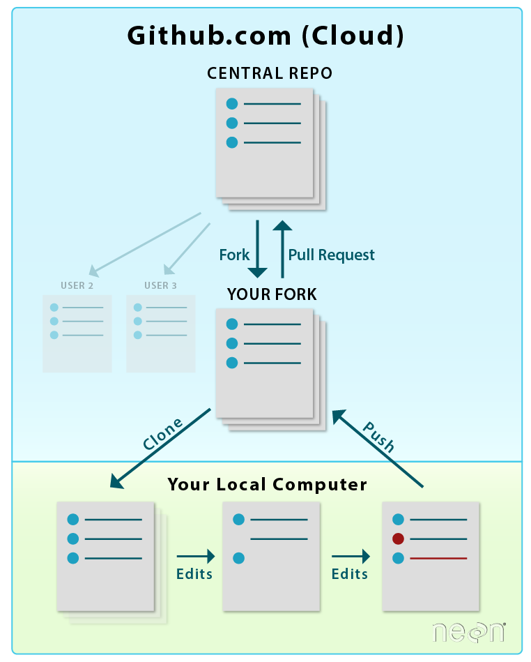
The distributed model of version control is where developers of code work from local repositories which are linked to a central repository. This enables automatic branching and merging, improves the ability to work offline, and doesn’t rely on a single repository for backup.
Git is the most popular open-source version control system among ecologists and also professional software developers. The popularity enables contributions from many collaborators since potential contributors will likely be used to using Git and web interfaces like GitHub.
You can practice using Git for version control with some simple tutorials.
GitLab also uses Git, and similar to GitHub allows for issue tracking and various other project management tools, and GitLab provides more options for collaborator authentication.
Example of version control workflow using Git. Figure from here.
Traditionally, scientific writing and coding are separate activities—for example, a researcher who wants to use code to generate a figure for her paper will have the code for generating that figure in one file and the document itself in another. This is a challenge for reproducibility and provenance tracking because both criteria have to be maintained for multiple files simultaneously. “Literate programming” provides an alternative approach, whereby code and text are interleaved within a single file; these files can be processed by special literate programming software to produce documents with the output of the code (e.g. figures, tables, and summary statistics) automatically interspersed with the document’s body text. This approach has several advantages. For one, the code output of a literate programming document is by definition guaranteed to be consistent with the code in the document’s source. At the same time, literate programming can make it easier to develop analyses by reducing the separation between writing and coding; for instance, interactive literate programming software can be used to keep “digital lab notebooks” where analyses are developed and described in the same file. In the context of ecological forecasting, literate programming techniques can be particularly useful for writing forecast software documentation, and can even be used for creating automatically-updating documents and reports describing forecast output.
Tools for literate programming
Two effective and common tools for literate programming are:
R Markdown — Allows code from multiple different languages including R, Python, SQL, C, and sh to be embedded within a common markup language (Markdown). Multiple different languages can be embedded within different blocks in the same document. Documents can be exported to a wide range of formats, including PDF, HTML, and DOCX. By default, R Markdown documents are static (i.e. the entire document is rendered all at once with a command); however, recent versions of RStudio allow them to be used interactively by rendering specific code blocks directly in the code editor window. R Markdown documents compiled to HTML format can easily embed interactive elements ranging from clickable plots and subsettable tables (e.g. htmlwidgets) to full applications with user-defined inputs (via RShiny); for more information, stay tuned for our follow up task view on Visualization.
Jupyter — Unlike R Markdown, these were designed from the start to be used interactively. Documents are stored in a format that makes them difficult to edit with a plain-text editor; rather, they are typically edited using a special browser-based editor that runs a language “kernel” in the background. The results of any particular code block are stored across sessions, so code blocks do not need to be re-evaluated when exporting to other formats. A document can only use a single language, with Julia, Python, and R supported.
Workflows are typically high-level descriptions of sets of tasks to be performed as part of an overall scientific application, at least in the context of this blog. There are a wide variety of methods and formats for expressing such descriptions. Workflows must include information about the tasks themselves, as well as their inputs and outputs, which either implicitly define or explicitly state dependencies among the tasks. This information, including the dependencies, is used by a Workflow Management System (WMS) to execute the tasks, potentially 1) on a local computer or one or more remote computers, including clouds and HPC or HTC systems; 2) serially or in parallel; 3) from the start or from a previous partially complete state. These dependencies can be static (fully defined before the application is run) or dynamic (e.g. partially defined based on data, execution, or other resources).
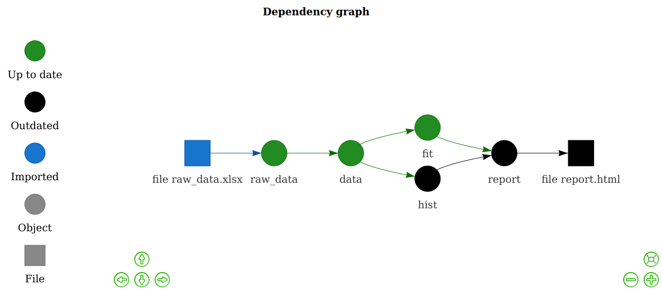
Workflow management systems help efficiently reproduce portions of or entire scientific workflows. These tools analyze workflows, skip phases of the workflow that are up-to-date (if the exact inputs and tasks have been run previously, the previous outputs can be returned; this technique is sometimes called memoization), and execute tasks that are out-of-date, tasks downstream of out-of-date tasks, or tasks required to execute based on scheduled run times (e.g., daily-updating forecast). These tools are especially useful for large projects that bring multiple streams of data together in an analysis since it relieves the analyst from duties of keeping track of workflow order and tasks that need to be rerun. For example, when new data about a model parameter is included in the forecasting workflow, only the portion of the workflow dependent on that new data will be executed.
Example of a simple dependency graph and which tasks will be executed using a workflow management system (from Drake workflow example).
Below we list a few tools for workflows and dependency management. There are however many other workflow and dependency management tools. A larger list can be found here.
Drake is an R-based ‘make’ like toolkit that tracks dependencies among phases of your workflow and executes work that is out-of-date. Drake builds upon previous R dependency managers such as remake, and can deal with high-performance or -throughput computing (HPC / HTC) within the WMS framework. This includes automated detection and retries for model failures, and launching Slurm (or other job schedulers for HTC) jobs directly from a drake plan.
Snakemake is a Python-based workflow management tool that includes a lot of the same functionality as Drake for R, including being compatible with HPC / HTC or cloud computing environments. The rules defined in a Snakemake target can use shell or Python commands or run external Python or R scripts, as well as utilize various remote storage environments such as Amazon S3, Dropbox, or Google Storage.
Parsl is a Python library that lets users define a workflow through a Python program, or parallelize a Python program. They do this by ‘decorating’ the definition of Python functions and calls to external applications to indicate that they are potentially parallelizable and asynchronous tasks. When such a task is called, Parsl intercepts it and adds it to an internal dynamic directed acyclic graph that captures the overall application dependencies. If both the inputs for the task and execution resources are available, the task is run, and if not, it waits until these conditions are satisfied. In either case, Parsl immediately returns a ‘future’, a placeholder for the eventual return value, so that the overall application can proceed, which allows multiple tasks to run in parallel. Parsl is an open source project led by U Chicago & Illinois, which supports a wide variety of execution resources (e.g., local, CPUs, GPUs, HPC, HTC, cloud) and schedulers.
Pegasus is another scientific workflow system with a long history of development and use in the science world (e.g., it’s the workflow system used by LIGO)
Argo is a more recent kubernetes-based workflow system, convenient when much of the workflow is within docker already (see Containerization below).
Airflow is another workflow system, developed and used by AirBnB and others, mostly in industry. Airflow is now a project within the Apache Software Foundation. It allows a user to author workflows as Directed Acyclic Graphs (DAGs) of tasks. The Airflow scheduler executes the tasks on an array of workers while following the specified dependencies. It also has a user interface to allow the user to visualize pipelines running in production, monitor progress, and troubleshoot issues.
Ecological forecasting workflows can be complex and involve many steps from data ingest, data cleaning, producing forecasts, to visualizing output. Often, these forecasting workflows need to produce output on a regular schedule and ensuring that each part of the workflow performs appropriately is crucial for making forecasts and identifying failure points, whether operational or not. Unit testing is automated tests on small units within a larger workflow to ensure that the different sections behave as intended (e.g. testing that individual functions return the expected outputs for valid inputs and the expected errors for invalid inputs). Frequently unit tests are also used for regression testing, where a test is created for a previous bug or problem that is fixed. The regression test is used to prevent a bug from being reintroduced. In combination with continuous integration (see below), these tests ensure that modifications to a code base run as expected after the modifications have been integrated.
In case of complex workflows or systems, a unit test will only test to make sure each of the components are working as intended. Additionally an integration or system test will need to be performed at certain points to test all the components interacting with each other. For example does each component still produce the outputs expected by the next steps in the workflow.
Tools for unit testing
Most programming languages have a testing framework that will help with the unit tests. A list of tools here, some of the commonly used testing frameworks for tools used in forecasting are:
testthat for R, including examples of how to implement unit testing in R.
Both the models we use to make predictions and the forecasting workflows we build around them are, in some sense, always a work in progress. Any time we make changes to our models and workflows, whether it’s updating a library or adding a data source, there’s a chance that we’ll break our workflow. Tools for continuous integration enable researchers to update their forecasts and run tests on their code in an automated and robust manner (e.g. with system tests in place to check for accidental deployments that would otherwise break a deployment). Continuous Integration (CI) tools automatically builds and deploys software ecosystems, and tests new versions of code to ensure development of models will work. This is especially important for iterative forecasts that need to be deployed at regular intervals (e.g. daily forecasts). As CI tools continue to become more powerful, flexible, and generous with their service offerings, they can expand from supporting development workflows to even be used as the primary platforms for application workflows, such as iterative, real-time forecasting. Below we list few of these tools and a larger list can be found here or here:
Travis CI, Probably the most popular automated testing tool on GitHub, at least in the recent past. This service is designed to test builds and run unit tests (and other, short-lived scripts) on a variety of different virtual platforms with different configurations. Travic CI runs for free on its Travis CI servers, but has time and CPU limits (at least for the free version (though a user can request that these limits be increased). Some features include the ability to run actions in parallel (configured via a YAML file) and an ability to be accessed via an API.
GitHub Actions, similar to Travis CI, but hosted natively by GitHub and with more generous time, memory, and CPU allowances for open-source (public) projects on GitHub. GitHub Actions is quickly increasing in popularity.
GitLab CI, similar to Travis and GitHub Actions but hosted by GitLab.
Complex scientific workflows often involve combining multiple different tools written in different programming languages and/or possessing different software dependencies. Even a simple R script may depend on multiple R packages, and may only work as expected if specific versions of those packages are used. Managing these different tools and their dependencies can be a complex task, especially when tools conflict with each other (e.g. one tool may only work with an older version of a library, while another tool may only work with a newer version of the same library). As the number of tools and their dependencies in a workflow grows, managing these dependencies becomes challenging, and reproducing this workflow on a different machine (potentially with a different operating system) is even more challenging. Containers resolve these issues by providing a way to create isolated packages for each software element and its dependencies. These containers can then run on any computing environment (as long as it has the requisite container software itself installed). Moreover, containerization software sometimes allows for the creation of container stacks (a.k.a “orchestration”)— collections of multiple containers that communicate with each other (including sharing data) and with the host system in precise, user-defined ways (see Workflow and Dependency Management above). In some cases, these container stacks can be deployed across multiple physical or virtual computers, which greatly facilitates the process of scaling computationally intensive analyses.
Tools for containerization
By far the most common tool for containerization — indeed, the emerging standard across the software development industry — is Docker. Docker containers are typically created from a definition file, basically just a starting container (e.g. a specific version of a Linux operating system) followed by a list of shell commands describing the installation and configuration of the specified software and its dependencies. Thousands of existing containers (any of which can be used as a starting point for a custom container) for a wide range of software are available on Docker Hub, a publicly available registry. Software stacks and workflows using multiple containers can be created via Docker Compose, which automatically configures and runs multiple interrelated Docker containers from a human-readable (YAML) specification file. Several tools for orchestration of Docker containers exist — Docker Swarm is distributed as part of Docker (i.e. no additional installation) and allows for rapid deployment with minimal configuration, while Kubernetes is a much more complex but feature-rich solution. Another quickly maturing tool leveraging Docker is The Binder Project, which is a relatively easy to use tool that turns a Git repository into a Docker image for deploying a reproducible computing environment in the cloud.
Unfortunately, Docker’s design precludes its use on high-performance computing clusters and other enterprise-managed machines often encountered in the sciences. In particular, running Docker containers requires running a persistent background process with administrative (“root”) privileges on the host machine. This is not an issue on self-managed, isolated physical (e.g. your personal laptop) and virtual (e.g. Amazon Web Services) machines. However, it does pose a major security concern that precludes its use on high-performance computing clusters and other enterprise-managed machines often encountered in the sciences. Singularity is an alternative that was designed specifically to address these concerns. Unlike Docker, Singularity does not require a persistent background process to run — rather, its design involves creating containers that are fully self-contained executable files. These files can then be distributed just like any other files, and executed on any machine (as long as that machine has a compatible version of Singularity installed). The initial install of Singularity, as well as the creation of containers, does require root permissions, but unlike Docker, the containers themselves run as a single process with only user permissions. Besides the security implications, this design also makes Singularity containers more amenable to HPC queue submission systems (running the containers is effectively the same as running any other executable). Like Docker, Singularity containers can be created via a definition file, and can be stored on a free, publicly available registry (Singularity Hub). The major downside of Singularity is that it has a much smaller user base (largely limited to a small subset of the scientific community, compared to Docker’s widespread use in both science and industry), and is much less mature software. For example, while Singularity does provide a “Compose” interface, as of this writing this is still in early development and highly experimental. Singularity also works with Kubernetes.
Metadata provide crucial information on the ecological forecasting data, including model input, output, and parameters, among others. Metadata tells the user how to interpret model output and what conditions are needed to reproduce output. Metadata is also used to describe the size and dimensions of the dataset, quality of the data, author of the data, keywords of the project used to produce the data, and details on how the data were produced. Appropriately documenting ecological forecasting output helps other researchers find relevant datasets and reuse output for other applications such as input to other models, or cross-model comparison such as a forecasting challenge.
Tools for metadata
Ecological Metadata Language (EML) is a community-maintained project for documenting research data with a readable XML markup syntax. EML serves the needs of the research community and is modularly designed to enable growth in the language as the needs of the earth and environmental sciences evolve. The Ecological Forecasting Initiative has developed additional forecast-specific standards using EML as the base metadata standards. The EML R package facilitates generating an EML document, however, these documents can also be created using a text editor or other scripting languages such as Python.
EFI is in the process of drafting an ecological forecasting metadata standard that extends EML. Current info is located in our forecast-standards repo
A core principle of creating reproducible scientific workflows is making the code and data used in the analyses available to the public through data and code publication or releases. It is now often required by journals or institutions to publish the data used in scientific publications and to a lesser extent, the code used in the analyses. Many of the other reproducible principles described above enable efficient data and code release and publication. For example, remote version control repositories, such as GitHub, display developmental and stable code bases and can tag versions of code to be released along with details on what the version was used for (e.g. “v1.2.1 used in analyses described by Dasari et al. 2019”). These code releases can also become citable with digital object identifier (DOI) by connecting with other archiving tools. Data releases should also be relatively painless if the previous principles of reproducible workflows are followed. Key to data releases and publishing in repositories are descriptive metadata that describe important characteristics of the dataset that is to be published (see Metadata section above). Additionally, embedding data publishing tasks (e.g. metadata descriptions, pushing data to a remote repository) in a dependency management system (see above) can make updating data in a public repository as easy as executing one line of code.
Tools for data and code release
Zenodo – a general purpose open-access repository, often used with GitHub to publish software.
DataOne – a repository for environmental and ecological data.
Dryad – a general purpose repository for research data.
Post by: Kathy Gerst1, Kira Sullivan-Wiley2, and Jaime Ashander3
Series contributors:
Mike Gerst4, Kailin Kroetz5, Yusuke Kuwayama6,
and Melissa Kenney7
1 USA National Phenology, 2Boston
University, 3Resources for the Future, 4University of Maryland, 5University of Arizona, 6Arizona State University, 7University of Minnesota
In this series, we are asking: How might ideas from the social sciences improve ecological forecasting? What new opportunities and questions does the emerging interdisciplinary field of ecological forecasting raise for the social sciences?This installment engages with the relationship between the people producing forecast outputs and the people interpreting those outputs.
First, it is important to note that some forecast products have a specific and known user (e.g., the EFI-affiliated Smart Reservoir project producing forecasts for the Western Virginia Water Authority). Others are produced for public use (e.g., weather forecasts) or by a wide range of potential users, some of whom may be known, but others not. This is important because there is variability in how people perceive, engage with, and understand visual products. This variability was seen in popular media in 2015 when the picture of a dress went viral and people could not agree on whether the dress was gold and white or black and blue. What people “see” can vary based on differences in not only neurology, but also personal experiences and perspectives. For forecasters, this means that we should never assume that a visual product that means one thing to us will automatically have the same meaning for the people using it.
Using social
science approaches to gain insights on how stakeholders perceive and use
forecast outputs can improve the ways in which model outputs are visualized and shared.
One example where people contribute to the design and refinement of forecasts comes from the USA National Phenology Network (USA-NPN; www.usanpn.org). The USA-NPN collects, stores, and shares phenology data and information to advance science and inform decisions. To do so, USA-NPN engages stakeholders, including natural resource managers and decision-makers, to guide the prioritization, selection, and development of data products and tools. This happens through a deliberate effort to engage and seek input from existing and new stakeholder audiences by cultivating relationships that can lead to collaborative teams and co-production of products. In this way, data users are actively involved throughout the process of scoping and developing projects that meet their needs.
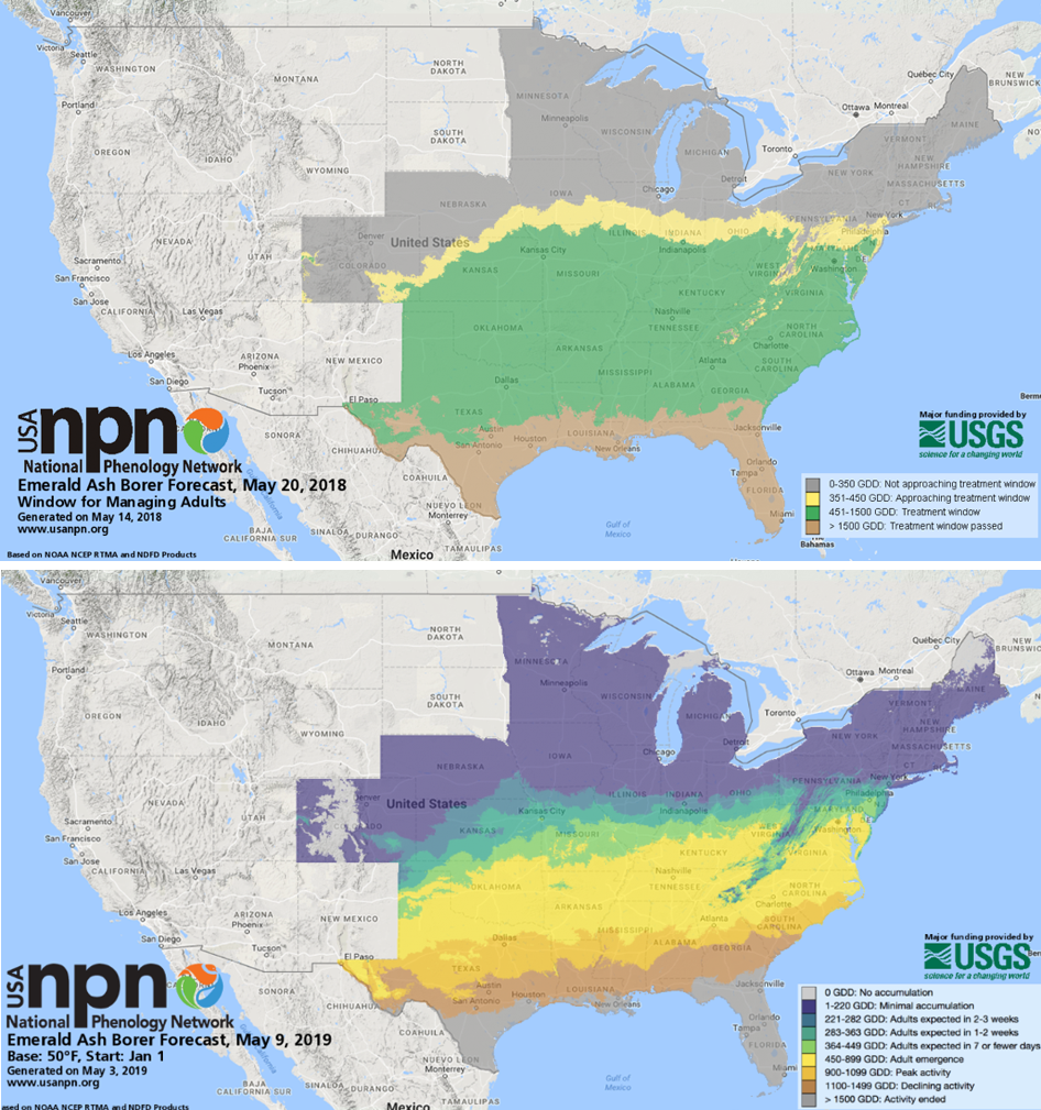
An example of a USA-NPN product designed with stakeholder input is the suite of Pheno Forecast maps (www.usanpn.org/data/forecasts); these maps show, up to 6 days in advance, when insect pests and invasive species are going to be in life stages that are susceptible to treatment. Interactions with end users after pilot maps were released revealed several opportunities for improvement.
Figure 1. The look and message of the Emerald Ash Borer Phenological Forecast produced by the USA National Phenology Network (USA-NPN) shifted substantially between 2018 (top) and 2019 (bottom) due to stakeholder feedback.
The original maps released in 2018 were focused on the “timing of treatment” –
that is, map categories portrayed locations based on whether they were
occurring before, during, or after particular treatment windows. Stakeholders
requested the visualized information
reflect life stages (e.g. eggs hatching or adults emerging) rather than
treatment window status (e.g. “approaching treatment window”), giving the end
user the opportunity to determine when (or if) to implement treatment (Figure 1). This visualization style also increased the
potential for the forecasts to be used by a broader community of people,
especially those with interests other than treatment.
In addition, some end users indicated that the original legend categories reflecting treatment window were too broad, and advocated for the use of narrower legend categories that allowed for more spatial differentiation among categories and more precise lead time before life stage transitions. Through consultation and the inclusion of stakeholders in the process, the NPN was able to harness the collective knowledge of the community to ultimately provide users with more nuanced and actionable information.
This case highlights both the importance of visualizations
in communicating forecast information and the importance of recognizing that
visualizations are more successful when they reflect a range of potential users
and uses. Approaches such as stakeholder participation and forecast
co-production are likely to increase the usability of forecast products and
their associated decision tools.
Further reading Additional resources will be updated in a living document that EFI is working to put together. We will add a link here once that goes live.
Academic Books and Articles Books by Denis Wood and co-authors on the ideologies, power dynamics, and histories embedded in maps. These accessible books may be particularly interesting for those interested in how visualizations (maps) can be harnessed by different people to establish or reclaim power, shape the human-environment relationship, or project a particular vision of reality.
Weaponizing
Maps (2015):
This book explores the “tension between military applications of participatory
mapping and its use for political mobilization and advocacy”
Rethinking
the Power of Maps (2010):
This book updates the 1992 “Power of Maps” and expands it by exploring “the
promises and limitations of diverse counter-mapping practices today.”
The
Natures of Maps (2008):
This book draws examples from maps of nature (or environmental phenomena) in
order to reveal “the way that each piece of information [visualized in the map]
collaborates in a disguised effort to mount an argument about reality” in ways
that can shape our relationship to the natural world.
The Power
of Maps (1992):
This book shows “how maps are not impartial reference objects, but rather
instruments of communication, persuasion, and power…[that] embody and project
the interests of their creators.”
Masuda (2009). Cultural Effects on Visual Perception. In book: Sage encyclopedia of perception, Vol. 1, Publisher: Sage Publications, Editors: In E. B. Goldstein (Ed, pp.339-343). link This chapter is a good overview of psychology research on how culture can influence what and how we “see.” It is full of research examples and is written in an accessible way.
Burkhard, “Learning from architects: the difference between knowledge visualization and information visualization,” Proceedings. Eighth International Conference on Information Visualisation, 2004. IV 2004., London, UK, 2004, pp. 519-524. IEEE link This paper is a quick and helpful overview of how a complement of tools can help us communicate either information or knowledge, drawing on tools used by architects (i.e. sketches, models, images/visions)
Chen et al. (2009) “Data, Information, and Knowledge in Visualization” IEEE. link This paper is a good reference for the distinctions among data, information, and knowledge, and how these can and should be treated differently in visualization products. Especially useful for those interested in distinctions in how these topics are treated in the cognitive and perceptual space as opposed to the computational space.
Blog posts on “best practices in data/information visualization” from data science companies Note: These practices underlie many of the visualizations produced and shared from the private sector and appear in advertising and media outlets—visualizations and visualization styles that will be familiar to most users of ecological forecasts
Series contributors: Mike Gerst3, Kathy Gerst4,5, Kailin Kroetz6, Yusuke Kuwayama2, and Melissa Kenney7
1Boston University, 2Resources for the
Future, 3University of Maryland, 4USA National Phenology Network,
5University of Arizona, 6Arizona
State University, 7University
of Minnesota
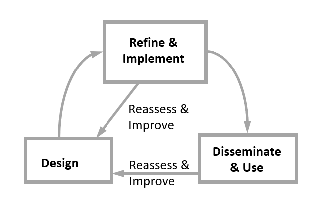
Ecological forecasting involves models and ecology but is
also a fundamentally people-centered endeavor. In their 2018 paper,
Mike Dietze and colleagues outlined the ecological forecasting cycle (Figure 1
is a simplified version of that cycle) where forecasts are designed, implemented,
disseminated, iteratively reassessed and improved through design. This cycle is about a process, and in each
part of this process there are people. Wherever there are people, there are
social scientists asking questions about them, their actions, and how to
improve decisions made by these insights.
So we ask the questions: How might ideas from the social
sciences improve ecological forecasting? What new opportunities and questions
does the emerging interdisciplinary field of ecological forecasting raise for
the social sciences?
This post introduces a series of posts that address these questions, discussing opportunities for the social sciences in Ecological Forecasting Initiative (EFI) and gains from considering humans in forecasting research. Thus, our aim is to better describe the role of social scientists in the ecological forecasting cycle and the opportunities for them to contribute to EFI.
Figure 1 The process of producing a forecast, which may begin at any step depending on which stakeholder group initiates.
So where are the people?
At EFI, we’re interested in reducing uncertainty of
forecasts, but also improving the processes by which we make forecasts that are
useful, useable, and used. This means improving forecasts, their design, use,
and impact, but it also results in a range of opportunities to advance basic
social science.
To do this we need to know: Where are the people in this
process? Where among the boxes and arrows of Figure 1 are people involved,
where do their beliefs, perceptions, decisions, and behavior make a difference?
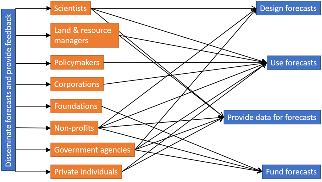
Are there people outside this figure who matter to the processes within it? Figure 2
highlights critical groups of people involved, and some of the actions they
take, that are integral to the ecological forecasting process.
Figure 2 Critical actors in the ecological forecasting process, linked with important actions
Figure 2 moves beyond the three-phase process described in
Figure 1 because the process of ecological forecasting is predicated on funding
sources and data, often provided by people and processes outside the
forecasting process. So when we think about where social science belongs in
ecological forecasting, we have to look beyond the forecasting process alone.
Making forecasts better
If EFI wants to make this process work and produce better
forecasts, which of these actors matters and how? How might different stakeholders
even define a “better” forecast?
One might think of “better” as synonymous with a lower degree of uncertainty,
while another might measure quality by a forecast’s impact on societal welfare.
Ease of use, ease of access, and spatial or temporal coverage are other metrics
by which to measure quality, and the relative importance of each is likely to
vary among stakeholders. Social science can help us to answer questions like:
Which attributes of a forecast matter most to which stakeholders, under what
conditions, and why?
While a natural scientist might assess the quality of a
forecast based on its level of uncertainty, a social scientist might assess the
value of a forecast by asking:
What individuals are likely to use the forecast?
How might the actions of these individuals change
based on the forecast?
How will this change in actions affect the
well-being of these or other individuals?
Building “better forecasts” will require a better
understanding of the variety of ways that stakeholders engage with forecasts.
The posts in this blog series will shine a spotlight on some of these
stakeholder groups and the social sciences that can provide insights for making
forecasts better. Posts in the series will discuss issues ranging from how
stakeholders interact with forecast
visualizations to the use of expert judgements in models to when forecasts
should jointly model human behavior and ecological conditions. Considering
these questions will help forecasters design forecasts that are more likely to
increase our understanding of these socio-environmental systems and enhance
societal well-being.
These examples hint at the range of potential interactions
between the social sciences and ecological forecasting. There is a wealth of
opportunity for social scientists to use the nascent field of ecological
forecasting to ask new and interesting questions in their fields. In turn, theories
developed in the social sciences have much to contribute to emerging
interdisciplinary practice of ecological forecasting in socio-environmental
systems. As we can see, better ecological forecasting may require us to think
beyond ecological systems.
My last blog briefly described the general process whereby new technologies and products are identified from the multitude available, culled, and eventually transitioned to operations to meet NOAA’s and its user’s needs, as well as offered some lessons learned when transitioning ecological forecasting products to operations, applications, and commercialization (R2X). In this blog, I introduce and briefly describe the steps in the R2X process used by NOAA’s Satellite & Information Service (NESDIS). NESDIS develops, generates, and distributes environmental satellite data and products for all NOAA line offices as well as for a wide range of Federal Government agencies, international users, state and local governments, and the general public. A considerable amount of planning and resources are required to develop and operationalize a product or service, and an orderly and well-defined review and approval process is required to manage the transition. The R2X process at NESDIS, managed by the Satellite Products and Services Review Board (SPSRB), is formal and implemented to identify funds and effectively manage the life cycle of a satellite product and service from development to its termination. It is a real-life example of how a science-based, operational agency transitions research to operations. A ‘broad brush’ approach of the process is given here, yet will hopefully be useful in providing insight into the major components involved in an R2X process that can be applied generally to the ecological forecasting (and other) communities. Details can be found in this SPSRB Process Paper.
The first step in the R2X process is acquiring a request for a new or improved product or service from an operational NOAA “user”. NESDIS considers requests from three sources: individual users, program or project managers, and scientific agencies. Individual users must be NOAA employees, so a relationship between a federal employee and other users, such as from the public and private sectors, including academia and local, state and tribal governments, must first be established. The request, submitted via a User Request Form similar to this one, must identify the need and benefits of the new or improved product(s) and includes requirements, specifications and other information to adequately describe the product and service. As an example, satellite-derived sea-surface temperature (SST), an operational product generated from several NOAA sensors, such as the heritage Advanced Very High Resolution Radiometer (AVHRR) and the current Visible Infrared Imaging Radiometer Suite (VIIRS), was requested by representatives from several NOAA Offices.
If
the SPSRB deems the request and its requirements valid and complete, the
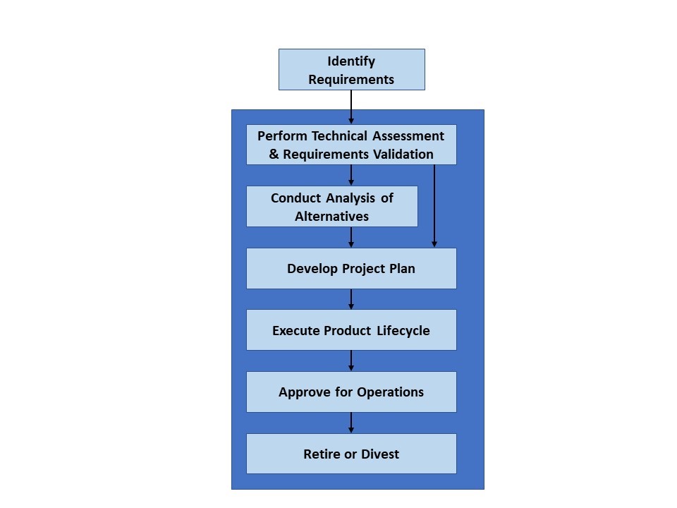
following six key steps are sequentially taken:
Perform Technical Assessment
Conduct Analysis of Alternatives
Develop Project Plan
Execute Product Lifecycle
Approve for Operations, and
Retire or Divest
These steps are depicted in Figure 1.
Figure 1. Key SPSRB process steps. Credit: Process Paper, Satellite Products and Services Review Board, 2018, SPSRB Improvement Working Group, Ver. 17, Department of Commerce. NOAA/NESDIS, 23 July 2018, 29pp.
1. Perform Technical Assessment and Requirements Validation
A technical assessment is performed to determine if the request is technically feasible, aligns with NOAA’s mission and provides management the opportunity to decide the best ways to process the user request. For instance, a user requests estimates of satellite-derived SST with a horizontal resolution of 1 meter every hour throughout the day for waters off the U.S. East Coast to monitor the position of the Gulf Stream. Though the request does match a NOAA mandate, i.e. to provide information critical to transportation, the specifications of the request are currently not feasible from space-borne sensors and the request would be rejected. On the other hand, a request for 1 km twice a day for the same geographic coverage would be accepted and the next step in the R2X process – Analysis of Alternative – would be initiated.
2. Conduct Analysis of Alternatives
An analysis of alternatives is performed to identify viable technical solutions and to select the most cost-effective approach to develop and implement the requested product or service that satisfies the operational need. An Integrated Product Team (IPT) consisting of applied researchers, operational personnel and users, is formed to complete this step. In the case of SST, this may be consideration of the use of data from one or more sensors to meet the user requests for the required frequency of estimates.
3. Develop Project Plan
The Project Plan describes
specifically how the product will transition from research to operations to
meet the user requirements following an existing template. Project plans are
updated annually. The plan consists of several important “interface processes”
that include:
Identifying resources to determine how the project will be funded. Various components of the product or services life cycle, from beginning to end, are defined and priced, e.g. support product development, long-term maintenance and archive. Though the SPSRB has no funding authority, it typically recommends the appropriate internal NOAA source for funding, e.g. the Joint Polar Satellite System Program;
Inserting the requirements of the product and service into an observational requirements list database for monitoring and record keeping;
Adding the product and service into an observing systems architecture database to assess whether observations are available to validate products or services, as all operational products and services must be validated to ensure that required thresholds of error and uncertainty are met; and,
Establishing an archiving capability to robustly store (including data stewardship) and to enable data discovery and retrieval of the requested products and services.
4. Execute Product Lifecycle
Product development implements the approved technical solution in accordance with the defined product or service capability, requirements, cost, schedule and performance parameters. Product development consists of three phases: development, pre-operational and operational. In the development stage, the IPT uses the Project Plan as the basis for directing and tracking development through several project phases or stages. In the pre-operations stage, the IPT begins routine processing to test and validate the product, including limited beta testing of the product by selected users. Importantly, user feedback is included in the process to help refine the product and ensure sufficient documentation and compatibility with requirements.
5. Approve for Operations
The NESDIS office responsible for operational generation of the product or service decides whether to transition the product or service to operations. After approval by the office, the IPT prepares and presents a decision brief to the SPSRB for it to assess whether the project has met the user’s needs, the user is prepared to use the product, and the product can be supported operationally, e.g. the infrastructure and sufficient funding for monitoring, maintenance, and operational product or service generation and distribution exists. The project enters the operations stage once the SPSRB approves the product or service. If the user identifies a significant new requirement or desired enhancement to an existing product, the user must submit a new user request.
6. Retire or Divest
If a product or service is no longer
needed and can be terminated, or the responsibility for production can be
divested or transferred to another organization, it enters the divestiture or
retirement phase.
Each of NOAA’s five Line Offices, e.g. Ocean Service, Weather Service, and Fisheries Service, has their own R2X process, that differs in one way or another to that of NESDIS. Even within NESDIS, if a project has external funding, it may not engage the SPSRB. Furthermore, the process may be updated if conditions justify, such as additional criteria are introduced from the administration. The process will, however, generally follow the major steps involved in the R2X process: user request, project plan, product/service development, implementation, product testing and evaluation, operationalization, and finally termination.
Acknowledgment: I thank John Sapper, David Donahue, and Michael Dietze for offering valuable suggestions that substantially improved an earlier version of this blog.
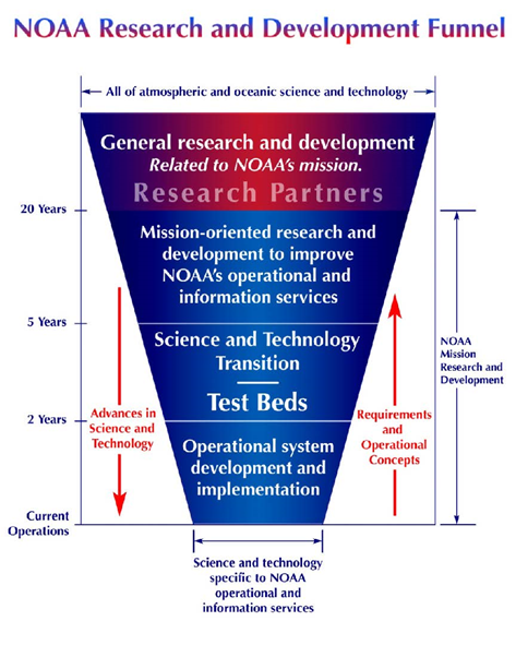
Ideally, newly developed ecological forecasts deemed useful should be transitioned to operations, applications or commercialization to benefit society. More succinctly, if there is no transition, there is no outcome. NOAA develops and transitions ecological forecasts to fulfill its mandates and role in the protection of life, property, human health and well-being, and in stewardship of coastal, marine, and Great Lakes environments. A depiction of this general process (Figure 1), affectionately called “the R&D funnel”, illustrates how new technologies and products are identified from the multitude available from numerous sources and are culled and eventually transitioned to meet NOAA’s needs. Unfortunately, while several ecological forecasting projects at NOAA have been successfully transitioned to operations, many projects remain primarily in a research mode. To better understand the reasons behind this, NOAA’s Ecological Forecasting Roadmap program conducted an unpublished study in 2014 that compared ecological forecasting projects that had been successfully transitioned to operations with those that languished or failed in order to identify common characteristics related to the success or failure of the transition. (NOAA defines operations as “sustained, systematic, reliable, and robust mission activities with an institutional commitment to deliver specified products and services”.) Based on the comparative analysis of nine projects, a list of “lessons learned” for transitioning ecological forecasts to operations, applications or commercialization (R2X) were compiled. The salient points are listed below:
Identify the “owner” or group responsible
for operationally producing the product or service as early as possible in the
process. In baseball vernacular, find
the catcher’s mitt;
Engage the users, stakeholders and
decision makers, from researchers to management, as early as possible to establish
user needs and obtain routine feedback for setting and updating product
requirements;
Find
and secure funding of the product or service to ensure its transition,
verification, sustainment and improvement;
Plan and document, to the best of
your ability, as many steps in the life of the product or service, from
research to operations to termination, including the entities responsible, the
major milestones, and the funding required. This activity will focus attention
on the steps that need to be taken and provide information required in the
formal R2X process; and
Include plans for the sustained collection,
analysis and archive of relevant data necessary for product verification.